Diffusion MRI Simulators: Hands-on Tutorial
Walk through DMRI's simulator API: build acquisition schemes, simulate single-compartment models (Ball/Stick), and mix them into multi-compartment signals.
import jax
import jax.numpy as jnp
import matplotlib.pyplot as plt

from dmri.simulators import Ball, MultiCompartment, Stick
from dmri.simulators.acquisition_scheme import acquisition_scheme
1. Build an acquisition scheme
acquisition_scheme bundles b-values (diffusion weighting) and b-vectors (gradient directions). We sample 100 directions on a unit sphere and linearly spaced b-values up to 3000 s/mm².
bvals = jnp.linspace(0, 3000, 100)
bvecs = jax.random.normal(jax.random.key(0), (100, 3))
bvecs = bvecs / jnp.linalg.norm(bvecs, axis=-1, keepdims=True)

acq = acquisition_scheme(bvals, bvecs)
acq
acquisition_scheme(bvals=Array([   0.     ,   30.30303,   60.60606,   90.90909,  121.21212,
        151.51515,  181.81818,  212.12122,  242.42424,  272.72726,
        303.0303 ,  333.33334,  363.63635,  393.9394 ,  424.24243,
        454.54544,  484.84848,  515.1515 ,  545.4545 ,  575.75757,
        606.0606 ,  636.36365,  666.6667 ,  696.96967,  727.2727 ,
        757.57574,  787.8788 ,  818.1818 ,  848.48486,  878.78784,
        909.0909 ,  939.3939 ,  969.69696, 1000.     , 1030.303  ,
       1060.6061 , 1090.909  , 1121.2122 , 1151.5151 , 1181.8181 ,
       1212.1212 , 1242.4242 , 1272.7273 , 1303.0303 , 1333.3334 ,
       1363.6364 , 1393.9393 , 1424.2424 , 1454.5454 , 1484.8485 ,
       1515.1515 , 1545.4546 , 1575.7576 , 1606.0605 , 1636.3636 ,
       1666.6666 , 1696.9697 , 1727.2727 , 1757.5757 , 1787.8788 ,
       1818.1818 , 1848.4849 , 1878.7878 , 1909.091  , 1939.3939 ,
       1969.6969 , 2000.     , 2030.303  , 2060.606  , 2090.9092 ,
       2121.2122 , 2151.5151 , 2181.818  , 2212.121  , 2242.4243 ,
       2272.7273 , 2303.0303 , 2333.3333 , 2363.6362 , 2393.9395 ,
       2424.2424 , 2454.5454 , 2484.8484 , 2515.1516 , 2545.4546 ,
       2575.7576 , 2606.0605 , 2636.3635 , 2666.6667 , 2696.9697 ,
       2727.2727 , 2757.5757 , 2787.8787 , 2818.182  , 2848.4849 ,
       2878.7878 , 2909.0908 , 2939.3938 , 2969.697  , 3000.     ],      dtype=float32), bvecs=Array([[ 0.61671704,  0.7697417 , -0.16479608],
       [-0.0793287 ,  0.17768422, -0.98088497],
       [-0.5132999 ,  0.51234627,  0.6884944 ],
       [-0.30866748,  0.70803624, -0.6351448 ],
       [ 0.26842725,  0.11812596,  0.9560299 ],
       [ 0.7979482 ,  0.51277804,  0.31676087],
       [ 0.00925005, -0.71769243, -0.69629884],
       [ 0.90436447,  0.02469544,  0.42604575],
       [ 0.10243183,  0.2206126 ,  0.96996796],
       [ 0.534678  , -0.62023616, -0.5739569 ],
       [-0.9811123 ,  0.19298749, -0.01320795],
       [ 0.43932244, -0.8556885 ,  0.27348316],
       [ 0.720231  , -0.6936246 , -0.01233524],
       [-0.12675364, -0.7582997 , -0.6394646 ],
       [ 0.38017547,  0.92362994,  0.0487268 ],
       [-0.2794273 , -0.2004503 , -0.93901014],
       [ 0.862728  ,  0.49443296,  0.10600198],
       [-0.02509449, -0.9586224 ,  0.28357252],
       [ 0.42645228,  0.71031475, -0.5599924 ],
       [ 0.77128434, -0.5506373 , -0.31924772],
       [-0.12770419, -0.29481807, -0.9469815 ],
       [ 0.48991367,  0.16495061, -0.85602325],
       [-0.5552431 ,  0.6804353 , -0.4782394 ],
       [ 0.50973666,  0.8250992 ,  0.24367973],
       [ 0.2831763 ,  0.7582117 ,  0.58730423],
       [ 0.769172  , -0.3437458 ,  0.53871447],
       [-0.00660573,  0.39260614, -0.919683  ],
       [ 0.8925746 ,  0.30049494,  0.33617467],
       [ 0.21295737,  0.10427797,  0.97148097],
       [ 0.37532106, -0.3714928 , -0.849192  ],
       [-0.6951644 ,  0.11984502,  0.7087903 ],
       [-0.6781298 ,  0.6846596 , -0.26717278],
       [-0.08840451, -0.5525801 ,  0.828758  ],
       [-0.5992693 ,  0.28025734,  0.74988806],
       [-0.02526362,  0.7414987 ,  0.6704785 ],
       [ 0.19262141, -0.63666755, -0.7466937 ],
       [-0.1016133 ,  0.97912025,  0.17606296],
       [ 0.21273269, -0.6569628 , -0.72328746],
       [ 0.53883797,  0.25268188, -0.8036203 ],
       [ 0.376659  ,  0.43198615, -0.8194608 ],
       [-0.50920206,  0.4229205 ,  0.74956757],
       [-0.89603764,  0.40378627, -0.18458943],
       [ 0.0826695 , -0.2066637 ,  0.9749133 ],
       [ 0.49653205,  0.62522435,  0.60212165],
       [-0.2085078 , -0.6174414 , -0.7584791 ],
       [ 0.22378272,  0.9500823 ,  0.21740513],
       [ 0.32094026, -0.11894663, -0.93960047],
       [-0.41179457,  0.18472844, -0.8923568 ],
       [ 0.17299542,  0.8756331 ,  0.45093155],
       [-0.68449515,  0.5365475 ,  0.49354145],
       [-0.6625935 ,  0.41354457,  0.62446034],
       [-0.5276852 , -0.37285045, -0.7632371 ],
       [-0.33758423, -0.26548764,  0.9030798 ],
       [-0.9197093 ,  0.2709466 ,  0.28411767],
       [ 0.06216538, -0.812555  , -0.57956004],
       [-0.31272247,  0.6043543 , -0.7327759 ],
       [-0.5183052 ,  0.36157826, -0.77499735],
       [ 0.8719175 , -0.3913285 , -0.29431593],
       [ 0.23578578, -0.46279752, -0.85453117],
       [-0.38656735, -0.91977894, -0.06761938],
       [-0.7038041 , -0.7094971 , -0.0356881 ],
       [-0.70036924,  0.06028405, -0.71123046],
       [ 0.7640203 , -0.2404989 , -0.5986929 ],
       [ 0.01514199,  0.35322204, -0.93541706],
       [ 0.8387477 , -0.54085726, -0.06305347],
       [ 0.51618785,  0.85594404, -0.03016751],
       [ 0.14058392,  0.98482835, -0.10173129],
       [ 0.7243224 ,  0.52242005,  0.44992703],
       [ 0.60533315, -0.77617735,  0.17641014],
       [-0.5711652 ,  0.76234317,  0.30430767],
       [-0.9679551 ,  0.23009104, -0.10060361],
       [-0.7405332 , -0.18883991,  0.6449419 ],
       [ 0.54774386,  0.57317257, -0.60946685],
       [-0.05314355, -0.12353322,  0.9909164 ],
       [-0.8833383 , -0.46691787,  0.04124564],
       [ 0.36258322,  0.54201525,  0.75812453],
       [-0.5868893 ,  0.6263565 , -0.5130677 ],
       [ 0.6432353 ,  0.60293937,  0.4719242 ],
       [ 0.11833139,  0.80322564,  0.5838033 ],
       [-0.7982449 ,  0.51824605, -0.3069625 ],
       [-0.28100488,  0.5779284 ,  0.76618207],
       [ 0.74551404, -0.6656686 ,  0.03307877],
       [-0.29239157, -0.73995066,  0.60578895],
       [-0.4093954 , -0.7642962 ,  0.49824363],
       [ 0.62949115, -0.55751354,  0.54122037],
       [-0.4201356 ,  0.2344518 , -0.8766518 ],
       [-0.6389138 ,  0.76543015, -0.07684909],
       [-0.05495164,  0.43374056, -0.89936054],
       [ 0.24537422, -0.47891432,  0.84287155],
       [-0.7668307 ,  0.3711711 , -0.52364373],
       [-0.07541212, -0.8555796 , -0.5121489 ],
       [ 0.77496874, -0.16022725, -0.6113515 ],
       [ 0.4348671 , -0.23283044, -0.8698739 ],
       [ 0.8146641 , -0.57387984,  0.083572  ],
       [ 0.79026335, -0.4608346 ,  0.40387517],
       [-0.00861309, -0.8188888 ,  0.5738876 ],
       [-0.984297  ,  0.14316551,  0.10326239],
       [ 0.07639609, -0.9855399 ,  0.15124369],
       [-0.2128922 , -0.44736174, -0.8686452 ],
       [-0.3218804 , -0.02440096, -0.94646585]], dtype=float32), delta=0.0106, Delta=0.0431)
2. Single-compartment examples
Ball: isotropic diffusion
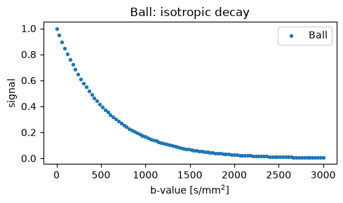
The Ball model represents free water with scalar diffusivity \(\lambda\).
lam = 0.0018  # mm^2/s
ball = Ball(lam)
ball_signal = ball.signal(acq)
fig, ax = plt.subplots(figsize=(5, 3))
ax.scatter(bvals, ball_signal, s=8, label="Ball")
ax.set(xlabel="b-value [s/mm$^2$]", ylabel="signal", title="Ball: isotropic decay")
ax.legend()
fig.tight_layout()
Stick: orientation dependence
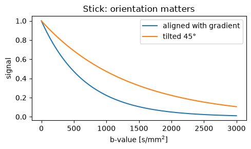
The Stick has zero radius and attenuates based on the projection of the gradient onto its orientation \(\boldsymbol{\mu}\).
# Orientation only shows up against a *fixed* gradient direction. With the
# random bvecs above, every point samples a different angle and the effect
# smears into a band, so build a single-direction scheme to see it cleanly.
acq_z = acquisition_scheme(bvals, jnp.tile(jnp.array([0.0, 0.0, 1.0]), (100, 1)))

stick_aligned = Stick(jnp.array([0.0, 0.0]), lam_par=0.0015)
stick_tilted = Stick(jnp.array([jnp.pi / 4, 0.0]), lam_par=0.0015)

signal_aligned = stick_aligned.signal(acq_z)
signal_tilted = stick_tilted.signal(acq_z)

fig, ax = plt.subplots(figsize=(5, 3))
ax.plot(bvals, signal_aligned, label="aligned with gradient")
ax.plot(bvals, signal_tilted, label="tilted 45$\\degree$")
ax.set(xlabel="b-value [s/mm$^2$]", ylabel="signal", title="Stick: orientation matters")
ax.legend()
fig.tight_layout()
3. Multi-compartment mixture
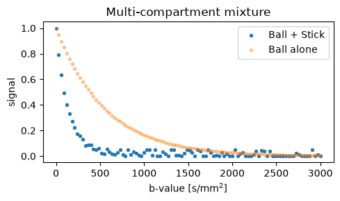
Combine compartments by subclassing MultiCompartment. Here we mix Ball + Stick with a uniform Dirichlet prior over fractions.
Noise compartments can be added separately to generate realistic magnitude observations.
class BallStick(MultiCompartment):
    model_types = [Ball, Stick]
    noise_types = []
    fraction_prior = jnp.ones(2)


theta = jax.random.normal(jax.random.key(123), (BallStick.theta_dim,))
model = BallStick.from_theta(theta)
signal_mix = model.signal(acq)
fig, ax = plt.subplots(figsize=(5, 3))
ax.scatter(bvals, signal_mix, s=8, label="Ball + Stick")
ax.scatter(bvals, ball_signal, s=8, alpha=0.4, label="Ball alone")
ax.set(xlabel="b-value [s/mm$^2$]", ylabel="signal", title="Multi-compartment mixture")
ax.legend()
fig.tight_layout()
4. Next steps
- Swap in
SphereorCylinderto explore restricted diffusion. - Add noise compartments (e.g.,
BoundedGaussianNoise) when simulating magnitude data. - Use
model_maskinMultiCompartment.from_thetato toggle components without changing the parameter layout.
For a deeper API tour, see the simulator guide.