Train a Small Model from Scratch
This notebook trains a deliberately small dMRI inference model in a few minutes on CPU. It uses the same simulator, model, and loss implementations as a full training run, but leaves out streaming data, checkpointing, WandB, and Hydra orchestration.
Every update receives a newly simulated batch, while a separate fixed batch measures held-out performance. The 25,000 updates process 1.6 million simulations in about one to two minutes on a modern CPU. The resulting model is still much smaller than a scientific checkpoint; see the training guide when you are ready for a full run.
import time

import jax
import jax.numpy as jnp
import matplotlib.pyplot as plt
import optax
from flax import nnx
from omegaconf import OmegaConf

from dmri.nn.autoregressive import DMRIModelSelectionAmortizedPriorConfig
from dmri.nn.dmri_reconstruction_model import (
    DMRIInferenceModel,
    DMRIInferenceModelConfigMaskPriorAmortizedPP,
)
from dmri.nn.embedding_net import DMRIEmbeddingConfig
from dmri.nn.simformer import DMRIThetaInferenceConfig
from dmri.train.build_simulator import build_simulator

print(jax.devices())
[CpuDevice(id=0)]
1. Build a small simulator
BallStick has only two possible signal compartments. Using 16 measurements keeps both simulation and attention inexpensive.
simulator_cfg = OmegaConf.create({
    "simulator": {
        "model_class": "dmri.simulators.models.BallStick",
        "posterior_score": False,
        "mask_prior": {"alpha": 1.0, "beta": 1.0},
        "acquisitions": [
            {
                "_target_": "dmri.simulators.random_clinical_acquisition",
                "_partial_": True,
                "num_acquisitions": 16,
            }
        ],
    }
})
sim_type, (simulator,) = build_simulator(simulator_cfg)
simulate_batch = jax.jit(jax.vmap(simulator))

batch_size = 64
validation_size = 256
validation_batch = simulate_batch(jax.random.split(jax.random.key(0), validation_size))
print({name: value.shape for name, value in validation_batch.items() if name != "acq"})
{'mask_prior': (256, 1), 'model_mask': (256, 2), 'theta': (256, 5), 'x': (256, 16)}
2. Build a tiny model
Production configurations use wider, deeper networks. Here every transformer has one layer and one attention head, giving a model small enough for an interactive example.
model_cfg = DMRIInferenceModelConfigMaskPriorAmortizedPP(
    simulator=sim_type,
    model_dim=16,
    embedding_cfg=DMRIEmbeddingConfig(
        num_layers=1, num_heads=1, widening_factor=2, attn_size=16
    ),
    model_selection_cfg=DMRIModelSelectionAmortizedPriorConfig(
        num_layers=1,
        num_heads=1,
        widening_factor=2,
        attn_size=16,
        prior_params_embed_dim=16,
    ),
    theta_inference_cfg=DMRIThetaInferenceConfig(
        num_layers=1,
        num_heads=1,
        widening_factor=2,
        attn_size=16,
        time_embed_dim=16,
    ),
)
model = DMRIInferenceModel(model_cfg, nnx.Rngs(0))
graphdef, params, model_state = nnx.split(model, nnx.Param, ...)

num_parameters = sum(x.size for x in jax.tree.leaves(params))
print(f"parameters: {num_parameters:,}")
parameters: 17,512
3. Train on fresh simulations
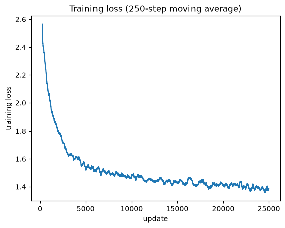
The model returns a model-selection loss and a parameter-inference loss. Each update below uses 64 newly simulated examples. The first update includes JAX compilation and is therefore much slower than the remaining updates.
optimizer = optax.adam(learning_rate=1e-3)
opt_state = optimizer.init(params)


@jax.jit
def update(params, model_state, opt_state, batch, rng):
    def loss_fn(params):
        train_model = nnx.merge(graphdef, params, model_state, copy=True)
        train_model.train()
        losses = train_model.loss_fn(rng, **batch, use_loss_mask=True)
        _, _, next_model_state = nnx.split(train_model, nnx.Param, ...)
        return losses.sum(), (losses, next_model_state)

    (loss, (losses, next_model_state)), grads = jax.value_and_grad(
        loss_fn, has_aux=True
    )(params)
    updates, opt_state = optimizer.update(grads, opt_state, params)
    params = optax.apply_updates(params, updates)
    return params, next_model_state, opt_state, loss, losses


@jax.jit
def evaluate(params, model_state, batch, rng):
    eval_model = nnx.merge(graphdef, params, model_state, copy=True)
    eval_model.eval()
    return eval_model.loss_fn(rng, **batch, use_loss_mask=True)


evaluation_rng = jax.random.key(2)
initial_validation_losses = evaluate(
    params, model_state, validation_batch, evaluation_rng
)
print(f"initial validation loss: {initial_validation_losses.sum():.3f}")

num_steps = 25_000
history = []
rng = jax.random.key(1)
started = time.perf_counter()
for step in range(num_steps):
    rng, simulation_rng, step_rng = jax.random.split(rng, 3)
    train_batch = simulate_batch(jax.random.split(simulation_rng, batch_size))
    params, model_state, opt_state, loss, losses = update(
        params, model_state, opt_state, train_batch, step_rng
    )
    history.append(loss)
    if step == 0 or (step + 1) % 2_500 == 0:
        print(
            f"step {step + 1:4d}: total={loss:.3f}, "
            f"mask={losses[0]:.3f}, theta={losses[1]:.3f}"
        )

history = jnp.asarray(history)
history.block_until_ready()
elapsed = time.perf_counter() - started
final_validation_losses = evaluate(
    params, model_state, validation_batch, evaluation_rng
)
print(f"final validation loss:   {final_validation_losses.sum():.3f}")
print(f"elapsed: {elapsed:.1f} seconds ({1_000 * elapsed / num_steps:.1f} ms/update)")

window = 250
smoothed_history = jnp.convolve(history, jnp.ones(window) / window, mode="valid")
plt.plot(jnp.arange(window, num_steps + 1), smoothed_history)
plt.xlabel("update")
plt.ylabel("training loss")
plt.title(f"Training loss ({window}-step moving average)")
plt.show()
initial validation loss: 6.957


step    1: total=7.436, mask=5.915, theta=1.521


step 2500: total=1.639, mask=0.336, theta=1.303


step 5000: total=1.425, mask=0.331, theta=1.094


step 7500: total=1.553, mask=0.332, theta=1.221


step 10000: total=1.436, mask=0.254, theta=1.182


step 12500: total=1.731, mask=0.343, theta=1.387


step 15000: total=1.420, mask=0.175, theta=1.245


step 17500: total=1.276, mask=0.234, theta=1.042


step 20000: total=1.241, mask=0.093, theta=1.148


step 22500: total=1.240, mask=0.193, theta=1.047


step 25000: total=1.611, mask=0.145, theta=1.466


final validation loss:   1.424
elapsed: 162.3 seconds (6.5 ms/update)
4. Evaluate held-out model selection
Reassemble the trained model and compare sampled masks with targets that were not used for optimization. This is a small synthetic validation set, but unlike training-batch accuracy it measures whether the model learned beyond individual examples.
trained_model = nnx.merge(graphdef, params, model_state, copy=True)
trained_model.eval()
predicted_masks = jax.vmap(trained_model.sample_mask, in_axes=(0, 0, 0, 0))(
    jax.random.split(jax.random.key(3), validation_size),
    validation_batch["acq"],
    validation_batch["x"],
    validation_batch["mask_prior"],
)

matches = predicted_masks == validation_batch["model_mask"]
print(f"component accuracy: {matches.mean():.3f}")
print(f"exact-mask accuracy: {matches.all(axis=-1).mean():.3f}")
print("first eight targets and predictions:")
print(jnp.c_[validation_batch["model_mask"][:8], predicted_masks[:8]].astype(int))
component accuracy: 0.930
exact-mask accuracy: 0.859
first eight targets and predictions:
[[1 0 1 0]
 [1 1 1 1]
 [1 1 1 1]
 [1 0 1 0]
 [1 0 1 0]
 [1 0 1 0]
 [0 1 1 1]
 [0 1 0 1]]
5. Sample the parameter posterior
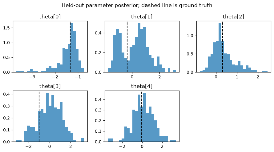
Choose a held-out example containing both compartments and draw parameter samples conditioned on its ground-truth mask. The dashed lines show the standardized parameters used to generate the observation. With this short training run, the marginals are only a qualitative check that the learned posterior covers plausible values.
sample_index = int(jnp.argmax(validation_batch["model_mask"].sum(axis=-1)))
acq = jax.tree.map(lambda value: value[sample_index], validation_batch["acq"])
x = validation_batch["x"][sample_index]
true_mask = validation_batch["model_mask"][sample_index]
true_theta = validation_batch["theta"][sample_index]

num_theta_samples = 256
theta_samples = jax.vmap(
    lambda key: trained_model.sample_theta(key, acq, x, true_mask, num_steps=32)
)(jax.random.split(jax.random.key(4), num_theta_samples))

posterior_mean = theta_samples.mean(axis=0)
print("mask:", true_mask.astype(int))
print(
    f"posterior-mean RMSE: {jnp.sqrt(jnp.mean((posterior_mean - true_theta) ** 2)):.3f}"
)

theta_dim = theta_samples.shape[-1]
fig, axes = plt.subplots(2, 3, figsize=(9, 5))
for index, ax in enumerate(axes.flat):
    if index >= theta_dim:
        ax.axis("off")
        continue
    ax.hist(theta_samples[:, index], bins=25, density=True, alpha=0.75)
    ax.axvline(true_theta[index], color="black", linestyle="--")
    ax.set_title(f"theta[{index}]")
fig.suptitle("Held-out parameter posterior; dashed line is ground truth")
fig.tight_layout()
plt.show()
mask: [1 1]
posterior-mean RMSE: 0.528
From notebook to full training
This is real online training, but it is intentionally small. For useful inference, use the Hydra training CLI described in the training guide. Full runs use larger model families, networks, and batches; maintain EMA parameters; evaluate more thoroughly; and save reproducible checkpoints.