Tutorial notebook. Source
.ipynb on GitHub.
Bayesian neural networks with probjax
A Bayesian neural network (BNN) puts a prior on the weights and, instead of a single fit, keeps the whole posterior over networks. Predictions average over it, so the spread of the predictive tells us where the model is unsure. That epistemic uncertainty should be small where we have data and grow where we do not.
This notebook samples the weight posterior of a small regression network in three ways and compares them:
- Full-batch HMC (
dynamic_hmc) with window warmup, four chains in parallel. - Convergence diagnostics (R-hat, ESS) — and why to compute them in function space.
- Stochastic-gradient MCMC (SGLD and SGHMC) on minibatches.
Every sampler runs through the same two calls, warmup and run.
import time

import jax
import jax.numpy as jnp
import matplotlib.pyplot as plt
from flax import nnx
from jax.scipy.stats import norm

from probjax.inference import run, warmup
from probjax.inference.diagnostics import effective_sample_size, rhat
from probjax.inference.mcmc import dynamic_hmc, sghmc, sgld
from probjax.inference.mcmc.sgmcmc import grad_estimator
from probjax.nn import MLP

jax.config.update("jax_platform_name", "cpu")
Data
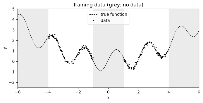
A 1D regression problem, \(y = 0.1x^2 + 0.1 + \sin(3x) + \varepsilon\) with \(\varepsilon \sim \mathcal{N}(0, 0.1^2)\). The 200 inputs come in two clusters, \([-4, -1]\) and \([1, 4]\), so there is a gap at \(|x| < 1\) and nothing beyond \(|x| > 4\). A good posterior should be confident on the clusters and uncertain in the gap and outside.
def true_fn(x):
    return 0.1 * x**2 + 0.1 + jnp.sin(3 * x)

num_data, noise_std = 200, 0.1
k_left, k_right, k_noise = jax.random.split(jax.random.key(0), 3)
X = jnp.concatenate([
    jax.random.uniform(k_left, (num_data // 2, 1), minval=-4.0, maxval=-1.0),
    jax.random.uniform(k_right, (num_data // 2, 1), minval=1.0, maxval=4.0),
])
Y = true_fn(X) + noise_std * jax.random.normal(k_noise, X.shape)
x_grid = jnp.linspace(-6, 6, 241)[:, None]

def plot_data(ax):
    ax.axvspan(-1, 1, color="0.92", zorder=0)
    for edge in (-6, 4):
        ax.axvspan(edge, edge + 2, color="0.92", zorder=0)
    ax.plot(x_grid, true_fn(x_grid), "k--", lw=1, label="true function")
    ax.plot(X, Y, "k.", ms=3, label="data")
    ax.set(xlim=(-6, 6), ylim=(-2.5, 5), xlabel="x", ylabel="y")

fig, ax = plt.subplots(figsize=(8, 3.5))
plot_data(ax)
ax.legend(loc="upper center")
ax.set_title("Training data (grey: no data)")
plt.show()
Model
A tanh MLP with two hidden layers of 16 units (321 weights) and a standard normal prior on every weight; the noise level is known.
Positions are a parameter pytree, not the module. nnx.split separates
the network into a static graphdef and an nnx.State holding the weights.
The state is an ordinary pytree of arrays, so the samplers can stack it over
chains and draws and jax.vmap over it directly; nnx.merge rebuilds a
callable network from any draw when we want predictions.
The log-likelihood is written for one data point. Full-batch HMC sums it
over the data; the stochastic-gradient estimator below rescales a minibatch
sum by num_data / batch_size.
def init_weights(seed):
    model = MLP([1, 16, 16, 1], activation=jnp.tanh, rngs=nnx.Rngs(seed))
    return nnx.split(model)

graphdef, weights = init_weights(0)
print("number of weights:", sum(w.size for w in jax.tree.leaves(weights)))

def predict(weights, x):
    return nnx.merge(graphdef, weights)(x)

def log_prior(weights):
    return sum(norm.logpdf(w).sum() for w in jax.tree.leaves(weights))

def log_likelihood(weights, datum):
    x, y = datum
    return norm.logpdf(y, predict(weights, x), noise_std).sum()

def log_posterior(weights):
    per_point = jax.vmap(log_likelihood, in_axes=(None, 0))(weights, (X, Y))
    return log_prior(weights) + per_point.sum()
number of weights: 321
Full-batch HMC with warmup
dynamic_hmc jitters the number of leapfrog steps from one transition to the
next (here around 50), which avoids the resonances of fixed-length HMC. Its
default adaptation is Stan-style window warmup, which tunes the step size and a
diagonal mass matrix; warmup picks it up automatically.
We run four chains from different random initialisations with jax.vmap.
Each chain adapts on its own: BNN chains usually settle in different modes,
so pooling their adaptation with pooled(adaptor) would mix up statistics from
unrelated regions of weight space.
num_chains, num_warmup, num_samples = 4, 2000, 1000
init_positions = jax.tree.map(
    lambda *w: jnp.stack(w), *[init_weights(seed)[1] for seed in range(num_chains)]
)
hmc_kernel = dynamic_hmc(log_posterior, average_integration_steps=50)

def hmc_chain(key, position):
    k_init, k_warm, k_run = jax.random.split(key, 3)
    state = hmc_kernel.init(k_init, position)
    warm = warmup(k_warm, hmc_kernel, state, hmc_kernel.init_params(state), num_warmup)
    collect = ("position", "logdensity", "acceptance_rate", "is_divergent")
    return run(k_run, hmc_kernel, warm.state, warm.params, num_samples, collect=collect)

start = time.perf_counter()
hmc = jax.jit(jax.vmap(hmc_chain))(jax.random.split(jax.random.key(1), num_chains), init_positions)
hmc = jax.block_until_ready(hmc)
hmc_seconds = time.perf_counter() - start
print(f"HMC: {num_chains} chains x {num_warmup} + {num_samples} steps in {hmc_seconds:.1f} s")
print("step size  ", hmc.params.step_size)
print("acceptance ", hmc.trace["acceptance_rate"].mean(axis=1))
print("divergences", hmc.trace["is_divergent"].sum(axis=1))
HMC: 4 chains x 2000 + 1000 steps in 31.7 s
step size   [0.00139759 0.00098797 0.00241417 0.00137113]
acceptance  [0.95973325 0.9774156  0.8174675  0.95463973]
divergences [0 0 0 0]
Diagnostics
The log posterior of each chain is a cheap first check: the chains should reach the same level and fluctuate around it.
R-hat and ESS on individual weights are not informative for a BNN. Permuting hidden units or flipping the sign of a tanh unit gives a different weight vector with the same function, so different chains legitimately sit in different, equivalent modes and weight-space R-hat is huge even when the predictions agree. What we care about is the function, so we compute R-hat and ESS of the network output \(f(x)\) at each input on a grid.
def function_draws(trace, x):
    # (chains, draws, len(x)) network outputs for every stored position
    return jax.vmap(jax.vmap(predict, (0, None)), (0, None))(trace["position"], x)[..., 0]

hmc_f = function_draws(hmc.trace, x_grid)
hmc_rhat = rhat(hmc_f, chain_axis=0, sample_axis=1)
hmc_ess = effective_sample_size(hmc_f, chain_axis=0, sample_axis=1)

fig, axes = plt.subplots(1, 3, figsize=(15, 3.5))
axes[0].plot(hmc.trace["logdensity"].T, lw=0.7)
axes[0].set(xlabel="draw", ylabel="log posterior", title="Trace per chain")
for ax, values, label in [(axes[1], hmc_rhat, "R-hat of f(x)"), (axes[2], hmc_ess, "ESS of f(x)")]:
    for lo, hi in [(-6, -4), (-1, 1), (4, 6)]:
        ax.axvspan(lo, hi, color="0.92", zorder=0)
    ax.plot(x_grid[:, 0], values, "C0")
    ax.set(xlabel="x", title=label, xlim=(-6, 6))
axes[1].axhline(1.01, color="k", ls=":", lw=1)
axes[2].set_yscale("log")
plt.tight_layout()
plt.show()

on_data = (jnp.abs(x_grid[:, 0]) > 1) & (jnp.abs(x_grid[:, 0]) < 4)
print(f"median R-hat on data: {jnp.median(hmc_rhat[on_data]):.3f}, off data: {jnp.median(hmc_rhat[~on_data]):.3f}")
print(f"median ESS   on data: {jnp.median(hmc_ess[on_data]):.0f}, off data: {jnp.median(hmc_ess[~on_data]):.0f}")
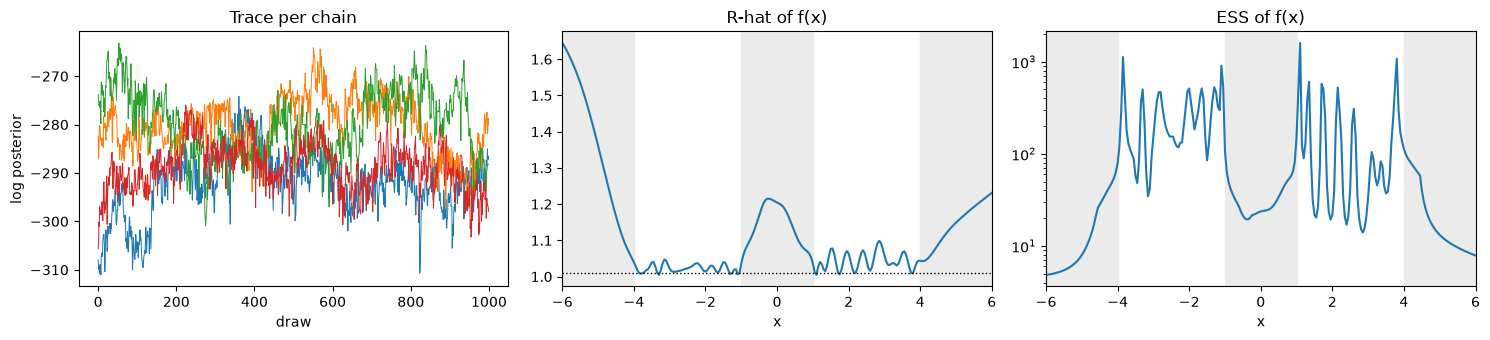
median R-hat on data: 1.028, off data: 1.171
median ESS   on data: 147, off data: 22
Where there is data, R-hat is close to 1 and the chains agree. In the gap and outside the data they do not: each chain explores one family of functions that fit the data equally well but extrapolate differently, and HMC moves between those families only slowly. Elevated R-hat off the data is therefore not a bug but the signature of a multimodal posterior. Several independent chains are what reveals it, and pooling their draws gives a better picture of the predictive uncertainty than any single chain.
Posterior predictive
Each draw is one network. Their mean is the prediction; their spread is the epistemic uncertainty. We also add the observation noise to get the predictive interval for new \(y\).
def plot_predictive(ax, f, color, title):
    draws = f.reshape(-1, f.shape[-1])
    mean, std = draws.mean(0), draws.std(0)
    total = jnp.sqrt(std**2 + noise_std**2)
    plot_data(ax)
    ax.plot(x_grid, draws[::200].T, color=color, lw=0.5, alpha=0.4)
    ax.fill_between(x_grid[:, 0], mean - 2 * total, mean + 2 * total, color=color, alpha=0.25, label="±2 std")
    ax.plot(x_grid, mean, color=color, lw=2, label="predictive mean")
    ax.set_title(title)

fig, ax = plt.subplots(figsize=(8, 4))
plot_predictive(ax, hmc_f, "C0", "HMC posterior predictive (thin lines: individual networks)")
ax.legend(loc="upper center", ncol=2)
plt.show()
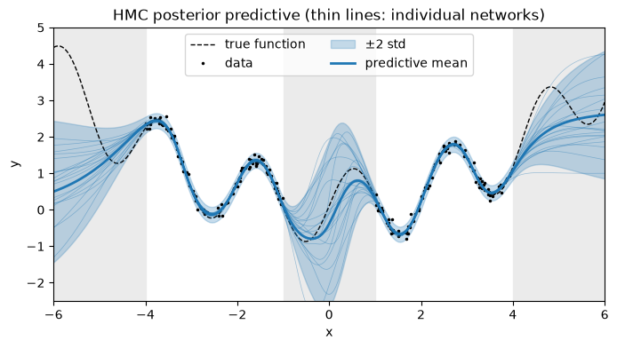
The predictive band hugs the data on the two clusters and widens in the gap and beyond \(|x| > 4\), exactly where the data says nothing.
Stochastic-gradient MCMC
Full-batch HMC evaluates the gradient on all 200 points at every leapfrog step, and its accept/reject step needs the exact log posterior. For large datasets that is too expensive. Stochastic-gradient MCMC replaces the gradient by a minibatch estimate,
and simulates Langevin (SGLD) or Hamiltonian (SGHMC) dynamics with it, without
a Metropolis correction. grad_estimator builds that estimate from our prior
and per-point likelihood.
Minibatches enter through run(..., args=...): each leaf of args has a
leading axis of length num_steps, and step \(t\) calls
kernel.step(key, state, params, minibatch_t). We draw each chain's batches
with replacement up front.
batch_size = 20
estimate_grad = grad_estimator(log_prior, log_likelihood, num_data)

def sg_chains(kernel, step_size, num_steps, key):
    def chain(key, position):
        k_batch, k_init, k_run = jax.random.split(key, 3)
        idx = jax.random.randint(k_batch, (num_steps, batch_size), 0, num_data)
        state = kernel.init(k_init, position)
        params = kernel.init_params(state, step_size=step_size)
        return run(k_run, kernel, state, params, num_steps, args=((X[idx], Y[idx]),), thin=num_steps // 1000)
    return jax.vmap(chain)(jax.random.split(key, num_chains), init_positions)

sg_chains = jax.jit(sg_chains, static_argnums=(0, 2))

def discard_burn_in(trace):
    # Without warmup the SG chains start from the random init: drop the first half.
    return jax.tree.map(lambda a: a[:, a.shape[1] // 2 :], trace)
SGLD and its step size
Without an accept/reject step, the step size controls a bias–variance trade-off: large steps mix faster but sample from a distorted, too-wide distribution, and beyond a stability limit (here around \(3 \cdot 10^{-5}\)) the chain diverges. There is no acceptance rate to adapt to, so we try a few step sizes and compare their draws with HMC, splitting the full-batch log posterior into its two terms.
sgld_kernel = sgld(estimate_grad)
sgld_steps = 100_000
sgld_runs, sgld_seconds = {}, {}
for step_size in [2e-6, 5e-6, 1e-5]:
    start = time.perf_counter()
    result = sg_chains(sgld_kernel, step_size, sgld_steps, jax.random.key(2))
    result = jax.block_until_ready(result)
    sgld_seconds[step_size] = time.perf_counter() - start
    sgld_runs[step_size] = discard_burn_in(result.trace)
    print(f"SGLD step size {step_size:.0e}: {num_chains} x {sgld_steps} steps in {sgld_seconds[step_size]:.1f} s")

def log_terms(trace):
    # Split the full-batch log posterior of every draw into data fit and prior.
    def terms(w):
        return jax.vmap(log_likelihood, (None, 0))(w, (X, Y)).sum(), log_prior(w)
    return jax.vmap(jax.vmap(terms))(trace["position"])

samples = {"HMC": hmc.trace} | {f"SGLD {h:.0e}": t for h, t in sgld_runs.items()}
fig, axes = plt.subplots(1, 2, figsize=(13, 3.5))
for color, (name, trace) in zip(["C0", "C3", "C1", "C4"], samples.items()):
    style = dict(color=color, alpha=0.6) if name == "HMC" else dict(color=color, histtype="step", lw=2)
    for ax, values, bins in zip(axes, log_terms(trace), [jnp.linspace(0, 200, 60), jnp.linspace(-500, -360, 60)]):
        ax.hist(values.ravel(), bins=bins, density=True, label=name, **style)
axes[0].set(xlabel="log likelihood (data fit)", ylabel="density")
axes[1].set(xlabel="log prior (weight size)")
axes[0].legend()
plt.show()
SGLD step size 2e-06: 4 x 100000 steps in 3.6 s


SGLD step size 5e-06: 4 x 100000 steps in 3.3 s


SGLD step size 1e-05: 4 x 100000 steps in 3.2 s
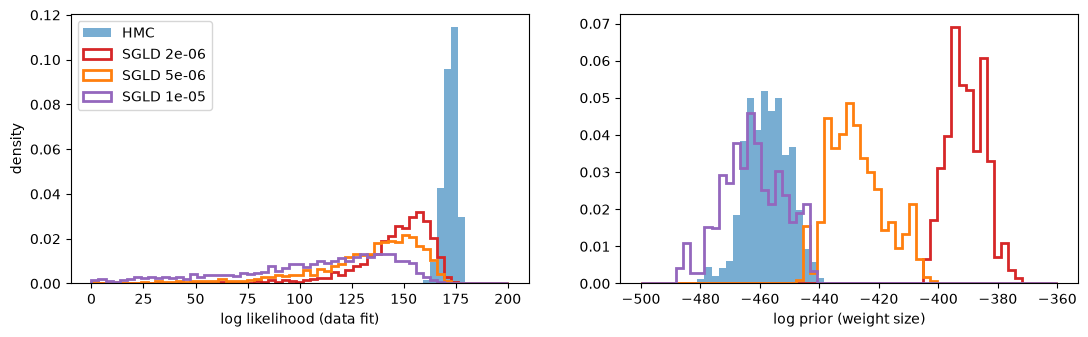
Neither panel is a clean win. Data fit (left): every SGLD run fits the data worse than HMC, and the larger the step, the longer the tail of poor fits — the minibatch gradient noise and the missing Metropolis correction both inflate the spread. Prior term (right): with small steps the weights have not yet spread out to the scale the prior allows. Those directions are barely constrained by the data and the chain drifts along them slowly; only the largest step size gets there in 100k steps. Small steps are accurate but slow, large steps are fast but biased. We keep \(5 \cdot 10^{-6}\) as the compromise.
SGHMC
SGHMC adds momentum: each transition draws a fresh momentum and runs a short
trajectory (here 10 steps) on one minibatch. Friction alpha matters a lot.
Minibatch gradients are noisy and every step adds that noise to the momentum,
so friction has to remove it again. With the default alpha=0.01 the chain
overheats and fits the data badly; alpha * step_size around 0.5 works here.
sghmc_kernel = sghmc(estimate_grad, num_integration_steps=10, alpha=500.0)
sghmc_steps = 10_000
start = time.perf_counter()
result = sg_chains(sghmc_kernel, 1e-3, sghmc_steps, jax.random.key(3))
result = jax.block_until_ready(result)
sghmc_seconds = time.perf_counter() - start
sghmc_trace = discard_burn_in(result.trace)
print(f"SGHMC: {num_chains} x {sghmc_steps} transitions x 10 steps in {sghmc_seconds:.1f} s")
SGHMC: 4 x 10000 transitions x 10 steps in 4.8 s
Comparing the predictives
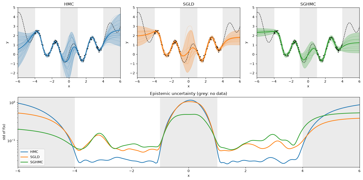
Same data, same model, three samplers. The bottom panel shows the epistemic standard deviation of \(f(x)\) along the input axis.
sgld_trace = sgld_runs[5e-6]
methods = {
    "HMC": (hmc_f, "C0"),
    "SGLD": (function_draws(sgld_trace, x_grid), "C1"),
    "SGHMC": (function_draws(sghmc_trace, x_grid), "C2"),
}

fig = plt.figure(figsize=(15, 7.5))
for i, (name, (f, color)) in enumerate(methods.items()):
    plot_predictive(fig.add_subplot(2, 3, i + 1), f, color, name)
ax = fig.add_subplot(2, 1, 2)
for lo, hi in [(-6, -4), (-1, 1), (4, 6)]:
    ax.axvspan(lo, hi, color="0.92", zorder=0)
for name, (f, color) in methods.items():
    ax.plot(x_grid[:, 0], f.reshape(-1, f.shape[-1]).std(0), color=color, lw=2, label=name)
ax.set(xlim=(-6, 6), xlabel="x", ylabel="std of f(x)", yscale="log", title="Epistemic uncertainty (grey: no data)")
ax.legend()
plt.tight_layout()
plt.show()
in_data = (jnp.abs(x_grid[:, 0]) > 1) & (jnp.abs(x_grid[:, 0]) < 4)
gap = jnp.abs(x_grid[:, 0]) < 1
datum_grads = {  # per-data-point gradient evaluations, all chains
    "HMC": num_chains * (num_warmup + num_samples) * 50 * num_data,
    "SGLD": num_chains * sgld_steps * batch_size,
    "SGHMC": num_chains * sghmc_steps * 10 * batch_size,
}
seconds = {"HMC": hmc_seconds, "SGLD": sgld_seconds[5e-6], "SGHMC": sghmc_seconds}
traces = {"HMC": hmc.trace, "SGLD": sgld_trace, "SGHMC": sghmc_trace}

print(f"{'':6} {'time [s]':>9} {'datum-grads':>12} {'log lik.':>10} {'RMSE on data':>13} {'std on data':>12} {'std in gap':>11}")
for name, (f, _) in methods.items():
    draws = f.reshape(-1, f.shape[-1])
    rmse = jnp.sqrt(jnp.mean((draws.mean(0) - true_fn(x_grid[:, 0])) ** 2, where=in_data))
    print(
        f"{name:6} {seconds[name]:9.1f} {datum_grads[name]:12.1e} {log_terms(traces[name])[0].mean():10.0f}"
        f" {rmse:13.3f} {draws.std(0)[in_data].mean():12.3f} {draws.std(0)[gap].mean():11.3f}"
    )
        time [s]  datum-grads   log lik.  RMSE on data  std on data  std in gap


HMC         31.7      1.2e+08        172         0.035        0.031       0.631
SGLD         3.3      8.0e+06        122         0.047        0.072       0.624
SGHMC        4.8      8.0e+06         73         0.062        0.089       0.349
All three samplers show the qualitative picture we want: small uncertainty on the clusters, large uncertainty in the gap and, for HMC and SGLD, growing uncertainty beyond \(|x| > 4\). The differences are in the details:
- On the data, the SG-MCMC predictives are two to three times wider than HMC's. That extra width is not epistemic uncertainty but sampler bias from noisy gradients and the missing Metropolis correction (compare the data-fit histogram above).
- Off the data, SGLD matches HMC in the gap but extrapolates more narrowly beyond the clusters; SGHMC is narrower in the gap as well. With only four chains, these off-data widths are themselves noisy (recall the R-hat there).
- Cost: the SG samplers used about 15 times fewer per-point gradient evaluations and a fraction of the wall time. Most of their time goes into many cheap steps, so the advantage grows with the dataset size.
Summary
- Setting up a BNN for probjax takes a log density over a weight pytree.
nnx.splitgives that pytree;nnx.mergeturns any draw back into a network for prediction. Writing the likelihood per data point lets the same model serve full-batch and minibatch samplers. - One API for every sampler.
warmupapplied the kernel's default window adaptation,runcollected positions and diagnostics, andjax.vmapran several chains; minibatches were justargs=. - Diagnose in function space. Weight-space R-hat is dominated by symmetries. Function-space R-hat is near 1 on the data and elevated in the gap and outside, where chains settle on different but equally plausible extrapolations. Use several chains and pool them.
- Epistemic uncertainty behaves as it should. All samplers are confident on the two clusters and uncertain in the gap and beyond \(|x| > 4\).
- SG-MCMC trades accuracy for cost. SGLD and SGHMC needed an order of magnitude fewer per-point gradients than HMC, but without a Metropolis correction they fit the data less tightly, inflate the uncertainty on the data, and depend on hand-tuned step size and friction. On a dataset this small, full-batch HMC is affordable and the more trustworthy reference; SG-MCMC pays off once full-batch gradients become the bottleneck.