Tutorial notebook. Source .ipynb on GitHub.

MCMC in probjax¶

Every MCMC algorithm in probjax.inference is a kernel: a pure transition step(key, state, params) -> (state, info) together with init and init_params. Three compiled functions drive any kernel:

Function	What it does
`run(key, kernel, state, params, num_steps, ...)`	scans the kernel, keeps the fields you `collect`, optionally adapts `params` while it runs
`warmup(key, kernel, state, params, num_steps, policy=None)`	fits the kernel parameters (step size, mass matrix, ...) with an adaptation policy
`step(key, kernel, state, params, adaptor=..., adaptor_state=...)`	one transition plus one adaptor update, for writing your own loop

This notebook walks through all of it:

running a chain and reading its trace,
a gallery of kernels on three hard 2D targets,
adaptation: default policies, composed adaptors, adapting while sampling and a custom adaptive loop,
many chains with shared (pooled) adaptation and convergence diagnostics,
pseudo-marginal MCMC for targets whose density can only be estimated.

Learned proposals and reparameterisations are covered in neural_mcmc.ipynb.

import time

import jax
import jax.numpy as jnp
import matplotlib.pyplot as plt
from jax.scipy.stats import norm

jax.config.update("jax_platform_name", "cpu")

from probjax.inference import (
    adjusted_mclmc,
    compose_adaptors,
    covariance_adaptor,
    ess_bulk,
    gauss_rwmh,
    gaussian_imh,
    hmc,
    mala,
    mclmc,
    nuts,
    pooled,
    pseudo_marginal,
    rhat,
    run,
    slice,
    step,
    step_size_adaptor,
    warmup,
)

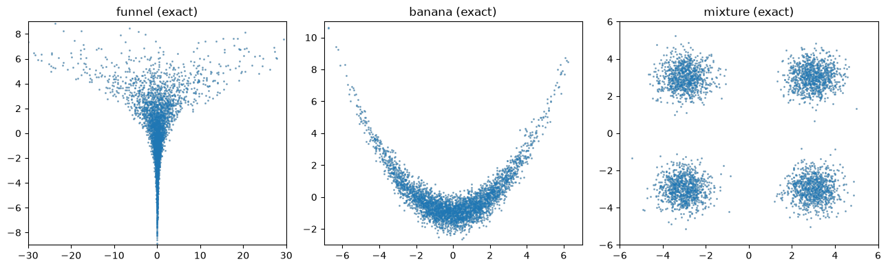
Three targets¶

Each target breaks a different assumption of a simple sampler:

Neal's funnel: the scale of x is exp(v / 2), so no single step size suits both the wide mouth and the narrow neck.
Banana: a strongly curved ridge, so the local correlation changes along it.
Mixture: four separated modes, so local moves rarely cross between them.

All three can be sampled exactly, which gives a reference to compare against.

def funnel_logdensity(z):
    x, v = z
    return norm.logpdf(v, 0.0, 3.0) + norm.logpdf(x, 0.0, jnp.exp(v / 2))


def banana_logdensity(z):
    x, y = z
    return norm.logpdf(x, 0.0, 2.0) + norm.logpdf(y, 0.25 * x**2 - 1.0, 0.5)


modes = jnp.array([[-3.0, -3.0], [-3.0, 3.0], [3.0, -3.0], [3.0, 3.0]])


def mixture_logdensity(z):
    log_components = norm.logpdf(z, modes, 0.6).sum(-1)
    return jax.scipy.special.logsumexp(log_components) - jnp.log(len(modes))


def exact_samples(name, key, n=20_000):
    k1, k2 = jax.random.split(key)
    e1, e2 = jax.random.normal(k1, (n,)), jax.random.normal(k2, (n,))
    if name == "funnel":
        v = 3.0 * e2
        return jnp.stack([jnp.exp(v / 2) * e1, v], -1)
    if name == "banana":
        x = 2.0 * e1
        return jnp.stack([x, 0.25 * x**2 - 1.0 + 0.5 * e2], -1)
    components = jax.random.randint(k1, (n,), 0, len(modes))
    return modes[components] + 0.6 * jax.random.normal(k2, (n, 2))


TARGETS = {
    "funnel": (funnel_logdensity, jnp.array([1.0, 0.0]), ((-30, 30), (-9, 9))),
    "banana": (banana_logdensity, jnp.array([0.0, -1.0]), ((-7, 7), (-3, 11))),
    "mixture": (mixture_logdensity, jnp.array([3.0, 3.0]), ((-6, 6), (-6, 6))),
}
REFERENCE = {
    name: exact_samples(name, jax.random.key(i)) for i, name in enumerate(TARGETS)
}


def scatter(ax, samples, name, title, color="C0"):
    reference = REFERENCE[name]
    ax.scatter(*reference[:4000].T, s=1, c="0.8", rasterized=True)
    ax.scatter(*samples.T, s=1, alpha=0.4, c=color, rasterized=True)
    xlim, ylim = TARGETS[name][2]
    ax.set(xlim=xlim, ylim=ylim, title=title)


fig, axes = plt.subplots(1, 3, figsize=(13, 4))
for ax, name in zip(axes, TARGETS):
    scatter(ax, REFERENCE[name][:4000], name, f"{name} (exact)")
plt.tight_layout()

png

Running a chain¶

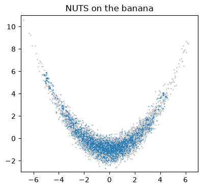
Build a kernel from the log density, initialise it at a position, tune its parameters with warmup and sample with run. Without a policy, warmup uses the kernel's own recommendation (kernel.default_adaptation), here Stan-style window adaptation of the step size and mass matrix.

collect names the state or info fields to keep at every retained step, and thin keeps every n-th transition.

kernel = nuts(banana_logdensity)
state = kernel.init(jax.random.key(0), jnp.array([0.0, -1.0]))
params = kernel.init_params(state)

tuned = warmup(jax.random.key(1), kernel, state, params, 1000)
result = run(
    jax.random.key(2),
    kernel,
    tuned.state,
    tuned.params,
    4000,
    collect=("position", "acceptance_rate", "num_integration_steps"),
    thin=2,
)

trace = result.trace
print("tuned step size:", tuned.params.step_size)
print("tuned inverse mass matrix:", tuned.params.inverse_mass_matrix)
print("kept draws:", trace["position"].shape)
print(f"mean acceptance: {trace['acceptance_rate'].mean():.2f}")
print(f"mean leapfrog steps per transition: {trace['num_integration_steps'].mean():.1f}")

fig, ax = plt.subplots(figsize=(4.5, 4))
scatter(ax, trace["position"], "banana", "NUTS on the banana")

tuned step size: 0.34944832
tuned inverse mass matrix: [2.318036   0.74416095]
kept draws: (2000, 2)
mean acceptance: 0.82
mean leapfrog steps per transition: 6.5

png

run is a single compiled scan. progress=True adds a progress bar with a moving average of the log density and acceptance rate (a tuple of names shows other state or info fields), and args= feeds per-step inputs such as minibatches.

Kernel gallery¶

Every kernel follows the same three steps, so comparing them is one loop. Each gets its default warmup (if it has one) and the same number of transitions. We report the bulk effective sample size of the worse coordinate and the wall time of the sampling run (compilation excluded). The per-transition cost differs a lot between kernels: random-walk and slice moves need no gradient, while HMC and NUTS take many gradient steps per transition.

KERNELS = {
    "RW-MH": gauss_rwmh,
    "Gaussian IMH": gaussian_imh,
    "Slice": slice,
    "MALA": mala,
    "HMC": hmc.configure(num_integration_steps=16),
    "NUTS": nuts,
    "MCLMC": mclmc,
    "Adjusted MCLMC": adjusted_mclmc,
}
NUM_WARMUP, NUM_SAMPLES = 1000, 4000


def sample(api, logdensity, position, key):
    kernel = api(logdensity)
    k_init, k_warm, k_run = jax.random.split(key, 3)
    state = kernel.init(k_init, position)
    params = kernel.init_params(state)
    if kernel.default_adaptation is not None:
        tuned = warmup(k_warm, kernel, state, params, NUM_WARMUP)
        state, params = tuned.state, tuned.params
    run(k_run, kernel, state, params, NUM_SAMPLES)  # compile
    start = time.perf_counter()
    draws = run(k_run, kernel, state, params, NUM_SAMPLES).trace["position"]
    draws.block_until_ready()
    return draws, time.perf_counter() - start


def modes_visited(draws):
    nearest = jnp.argmin(((draws[:, None] - modes) ** 2).sum(-1), -1)
    return int((jnp.bincount(nearest, length=len(modes)) > 0.01 * len(draws)).sum())


gallery = {}
for kernel_name, api in KERNELS.items():
    for target_name, (logdensity, position, _) in TARGETS.items():
        draws, seconds = sample(api, logdensity, position, jax.random.key(3))
        ess = float(ess_bulk(draws[None]).min())
        gallery[kernel_name, target_name] = (draws, ess, seconds)

print(f"{'kernel':<15}" + "".join(f"{t:>20}" for t in TARGETS) + "   mixture")
print(f"{'':<15}" + "".join(f"{'ESS  time [ms]':>20}" for _ in TARGETS) + "     modes")
for kernel_name in KERNELS:
    row = "".join(
        f"{gallery[kernel_name, t][1]:>10.0f}{1e3 * gallery[kernel_name, t][2]:>10.0f}"
        for t in TARGETS
    )
    visited = modes_visited(gallery[kernel_name, "mixture"][0])
    print(f"{kernel_name:<15}{row}{visited:>7}/4")

kernel                       funnel              banana             mixture   mixture
                     ESS  time [ms]      ESS  time [ms]      ESS  time [ms]     modes
RW-MH                 153        15       156        16        20        16      2/4
Gaussian IMH          288        18       232        15      3077        15      1/4
Slice                 128        61       163        56         2        59      2/4
MALA                   10        14        57        15      1776        17      1/4
HMC                   310        30      1255        17        84        23      1/4
NUTS                   49        95       226        89      3759        61      1/4
MCLMC                  10        54        84        60      1149        65      1/4
Adjusted MCLMC         96       136      1244       114      1311       128      1/4

fig, axes = plt.subplots(len(KERNELS), 3, figsize=(11, 3.2 * len(KERNELS)))
for row, kernel_name in zip(axes, KERNELS):
    for ax, target_name in zip(row, TARGETS):
        draws, ess, _ = gallery[kernel_name, target_name]
        scatter(ax, draws, target_name, f"{kernel_name}: {target_name} (ESS {ess:.0f})")
plt.tight_layout()

png

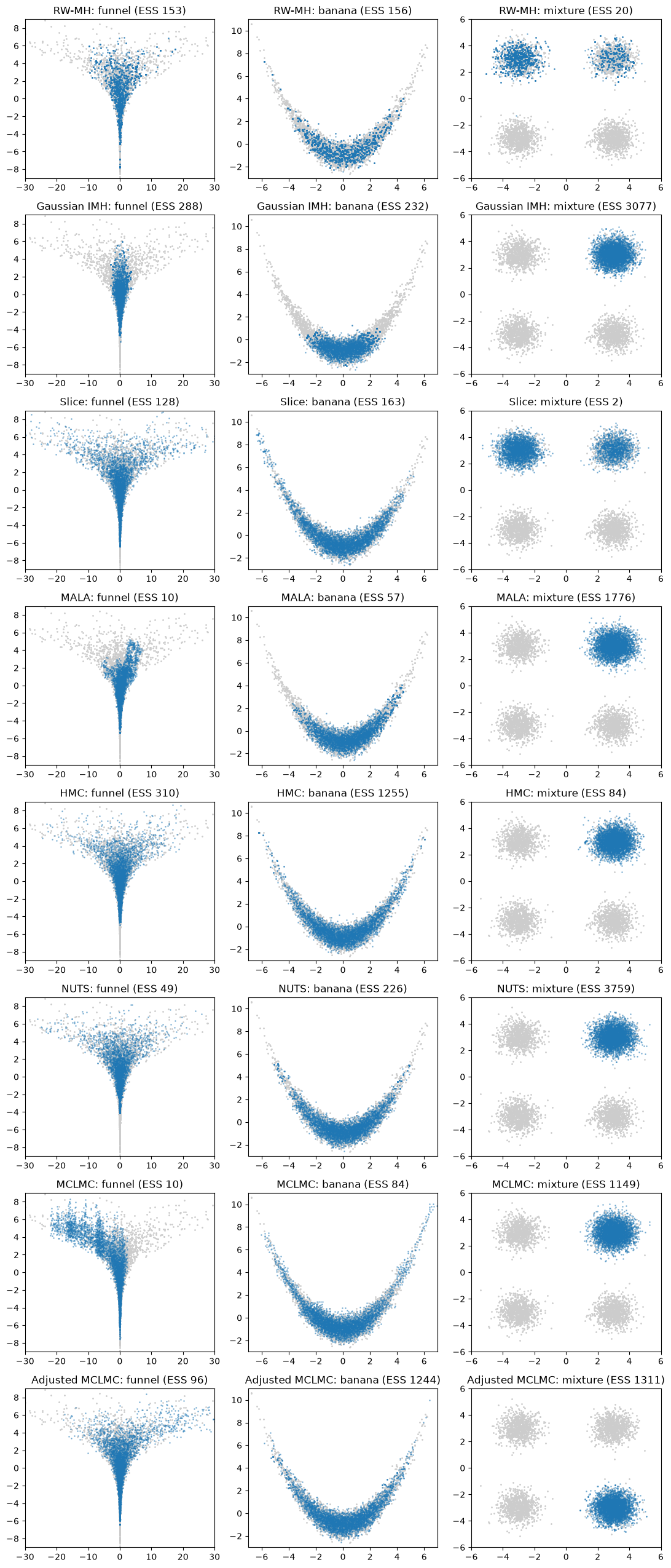
What the gallery shows (grey: exact samples; details vary with the seed):

Funnel. The mouth (large v) and the neck (very negative v) need step sizes orders of magnitude apart. Slice sampling, whose bracket adapts to every slice, covers the mouth as well as HMC, NUTS and adjusted MCLMC do, without a single gradient. No kernel gets deep into the neck within this budget, and the random walk, the Gaussian independence sampler, MALA and unadjusted MCLMC are visibly biased. This is the case for a learned reparameterisation (NeuTra, see neural_mcmc.ipynb).
Banana. The gradient methods and slice sampling follow the curved arms. A Gaussian independence proposal cannot cover a curved ridge and misses them.
Mixture. No kernel finds all four modes. The random walk and slice sampler occasionally step to a neighbouring mode; everything else stays where it started. Note the large ESS of chains that never left their mode: ESS measures how well a chain mixes within what it explored, not whether it explored everything. Several chains and \(\hat R\) (below) catch this; reaching all modes needs population methods (SMC, smc.ipynb) or a proposal that knows about them (neural IMH).

Adaptation¶

An adaptation policy is one of two things:

an Adaptor (init, update, finalize), a local state machine updated after every transition (dual averaging of the step size, Welford estimates of a covariance, ...). Adaptors compose and can run during warmup or sampling;
a Warmup, a self-contained procedure with its own schedule (Stan's window adaptation, Pathfinder, MCLMC's tuning).

Each kernel names its recommended policy:

for kernel_name, api in KERNELS.items():
    kernel = api(banana_logdensity)
    policy = kernel.default_adaptation and kernel.default_adaptation()
    print(f"{kernel_name:<15} {type(policy).__name__}")

RW-MH           Warmup
Gaussian IMH    Adaptor
Slice           Adaptor
MALA            Adaptor
HMC             Warmup
NUTS            Warmup
MCLMC           Warmup
Adjusted MCLMC  Adaptor

Composing adaptors¶

compose_adaptors threads several adaptors through the same parameters, in order. For a random walk on a 10-dimensional Gaussian with scales 1 to 10 we tune the step size towards the classic 0.234 acceptance rate and estimate the proposal scale from the chain.

One subtlety: a covariance estimate only enters the parameters when its adaptor is finalized, at the end of the warmup. The step size tuned alongside it therefore fits the old scale. A second, step-size-only phase fixes that; this two-phase schedule is gauss_rwmh's default warmup.

scales = jnp.linspace(1.0, 10.0, 10)
kernel = gauss_rwmh(lambda x: -0.5 * jnp.sum((x / scales) ** 2))
state = kernel.init(None, jnp.zeros(10))
params = kernel.init_params(state)

adaptor = compose_adaptors(
    step=step_size_adaptor(target=0.234),
    scale=covariance_adaptor(output="standard_deviation"),
)
composed = warmup(jax.random.key(4), kernel, state, params, 4000, adaptor)
two_phase = warmup(
    jax.random.key(4),
    kernel,
    composed.state,
    composed.params,
    4000,
    step_size_adaptor(target=0.234),
)
print("estimated scales:", jnp.round(composed.params.scale, 1))

collect = ("position", "acceptance_rate")
for label, p in [
    ("untuned", params),
    ("composed", composed.params),
    ("+ step size", two_phase.params),
]:
    out = run(jax.random.key(5), kernel, two_phase.state, p, 20_000, collect=collect)
    ess = ess_bulk(out.trace["position"][None]).min()
    print(
        f"{label:>12}: step size {p.step_size:.2f}, "
        f"acceptance {out.trace['acceptance_rate'].mean():.3f}, worst ESS {ess:.0f}"
    )

estimated scales: [1.1       2.1000001 3.        3.5       5.1       6.3       6.4
 7.6       7.2000003 8.7      ]


     untuned: step size 0.50, acceptance 0.784, worst ESS 17
    composed: step size 2.53, acceptance 0.003, worst ESS 3


 + step size: step size 0.88, acceptance 0.212, worst ESS 463

The 0.234 target is optimal for random walks on high-dimensional, roughly Gaussian targets. On strongly curved targets such as the banana, a larger step (lower acceptance) can mix better; the target is a knob, not a law.

Adapting while sampling¶

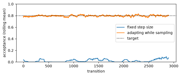
Passing adaptor= to run updates the parameters after every transition and returns the adaptor's finalized parameters. Here MALA starts with a step size that is far too large; the running acceptance rate shows dual averaging pulling it towards the 0.8 target within a few hundred transitions.

Adapting changes the transition kernel as it goes, so for draws you want to keep, either stop adapting (sample with the returned params) or use an adaptation that diminishes over time, as dual averaging does.

kernel = mala(banana_logdensity)
state = kernel.init(None, jnp.array([0.0, -1.0]))
params = kernel.init_params(state, step_size=3.0)

adaptive = run(
    jax.random.key(6),
    kernel,
    state,
    params,
    3000,
    adaptor=step_size_adaptor(target=0.8),
    collect=("acceptance_rate",),
)
fixed = run(jax.random.key(6), kernel, state, params, 3000, collect=("acceptance_rate",))
print(f"step size: {params.step_size:.3f} -> {adaptive.params.step_size:.3f}")


def rolling_mean(x, width=100):
    return jnp.convolve(x, jnp.ones(width) / width, mode="valid")


fig, ax = plt.subplots(figsize=(7, 3))
ax.plot(rolling_mean(fixed.trace["acceptance_rate"]), label="fixed step size")
ax.plot(rolling_mean(adaptive.trace["acceptance_rate"]), label="adapting while sampling")
ax.axhline(0.8, c="k", ls=":", label="target")
ax.set(xlabel="transition", ylabel="acceptance (rolling mean)", ylim=(0, 1))
ax.legend()
plt.tight_layout()

step size: 3.000 -> 0.138

png

Your own adaptive loop with `step`¶

step is one transition plus one adaptor update, so any control flow is a few lines. This warmup has no fixed length: it adapts until a moving average of the acceptance rate has settled at the target (with a cap), then finalizes.

kernel = mala(funnel_logdensity)
state = kernel.init(None, jnp.array([1.0, 0.0]))
params = kernel.init_params(state)
adaptor = step_size_adaptor(target=0.8)
warmup_key = jax.random.key(7)


@jax.jit
def adapt_until_settled(state, params):
    def keep_going(carry):
        i, *_, average = carry
        return (i < 5000) & ((i < 200) | (jnp.abs(average - 0.8) > 0.02))

    def one_step(carry):
        i, state, params, adaptor_state, average = carry
        state, params, adaptor_state, info = step(
            jax.random.fold_in(warmup_key, i),
            kernel,
            state,
            params,
            adaptor=adaptor,
            adaptor_state=adaptor_state,
        )
        average = 0.98 * average + 0.02 * info.acceptance_rate
        return i + 1, state, params, adaptor_state, average

    carry = (0, state, params, adaptor.init(state, params), 0.0)
    num_steps, state, params, adaptor_state, average = jax.lax.while_loop(
        keep_going, one_step, carry
    )
    params, _ = adaptor.finalize(adaptor_state, params)
    return num_steps, state, params, average


num_steps, state, params, average = adapt_until_settled(state, params)
print(f"settled after {int(num_steps)} transitions (acceptance {average:.2f}),"
      f" step size {params.step_size:.3f}")

settled after 208 transitions (acceptance 0.78), step size 0.045

Many chains¶

Chains are just jax.vmap over run. Give the vmap an axis_name and wrap the adaptor in pooled to adapt all chains as one: after every update the adaptor statistics are averaged over chains, so every chain ends with the same parameters, estimated from all of them.

Several chains from dispersed starting points are also what convergence diagnostics need. The rank-normalised \(\hat R\) compares chains with each other: it is close to 1 when they agree and large when they explore different regions.

def many_chains(logdensity, starts, key, adaptor):
    kernel = mala(logdensity)
    states = jax.vmap(lambda x: kernel.init(None, x))(starts)
    params = jax.vmap(kernel.init_params)(states)
    k_warm, k_run = jax.random.split(key)

    def one_chain(key_warm, key_run, state, params):
        tuned = run(key_warm, kernel, state, params, 1000, adaptor=adaptor, collect=())
        return run(key_run, kernel, tuned.state, tuned.params, 4000), tuned.params

    num_chains = len(starts)
    return jax.vmap(one_chain, axis_name="chain")(
        jax.random.split(k_warm, num_chains),
        jax.random.split(k_run, num_chains),
        states,
        params,
    )


starts = 4.0 * jax.random.normal(jax.random.key(8), (4, 2))
for label, adaptor in [
    ("independent", step_size_adaptor()),
    ("pooled", pooled(step_size_adaptor())),
]:
    _, chain_params = many_chains(banana_logdensity, starts, jax.random.key(9), adaptor)
    print(f"{label:>12} step sizes: {chain_params.step_size}")

diagnostics = {}
for name in ("banana", "mixture"):
    chains, _ = many_chains(
        TARGETS[name][0], starts, jax.random.key(9), pooled(step_size_adaptor())
    )
    draws = chains.trace["position"]  # (chains, draws, 2)
    diagnostics[name] = draws
    print(f"{name:>8}: R-hat {rhat(draws)}, bulk ESS {ess_bulk(draws)}")

 independent step sizes: [0.08298066 0.12210048 0.11154567 0.11171739]


      pooled step sizes: [0.11693113 0.11693113 0.11693113 0.11693113]


  banana: R-hat [1.0287931 1.0068477], bulk ESS [120.03735 369.3163 ]


 mixture: R-hat [1.52818  1.733971], bulk ESS [7.1396494 6.059352 ]

fig, axes = plt.subplots(1, 2, figsize=(12, 3))
for ax, name in zip(axes, diagnostics):
    for chain in diagnostics[name]:
        ax.plot(chain[:, 0], lw=0.5)
    ax.set(title=f"{name}: first coordinate of 4 chains", xlabel="draw")
plt.tight_layout()

png

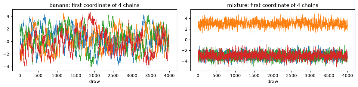
On the banana the chains overlap and \(\hat R \approx 1\). On the mixture each chain is stuck in the mode nearest to its start, and \(\hat R\) flags it clearly even though every single chain looks perfectly stationary on its own.

Pseudo-marginal MCMC¶

Sometimes the density can only be estimated, for example a likelihood with latent variables integrated out by Monte Carlo. If the estimate of the likelihood is unbiased, MCMC that keeps the estimate of the current state (instead of recomputing it) still targets the exact posterior. pseudo_marginal wraps any kernel this way; the log-density function takes a random key.

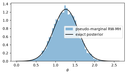
Model: \(y_j = \theta + z_j + \varepsilon_j\) with \(z_j, \varepsilon_j \sim \mathcal N(0, 1)\) and prior \(\theta \sim \mathcal N(0, 3^2)\). We pretend the marginal \(y_j \sim \mathcal N(\theta, 2)\) is unknown and estimate it by importance sampling over \(z\), then compare against the exact posterior.

theta_true, num_obs, num_particles = 1.5, 20, 64
y = theta_true + jnp.sqrt(2.0) * jax.random.normal(jax.random.key(10), (num_obs,))


def estimated_logdensity(theta, key):
    z = jax.random.normal(key, (num_particles, num_obs))
    log_weights = norm.logpdf(y, theta[0] + z, 1.0)  # (particles, observations)
    log_likelihood = jax.scipy.special.logsumexp(log_weights, 0) - jnp.log(num_particles)
    return norm.logpdf(theta[0], 0.0, 3.0) + log_likelihood.sum()


kernel = pseudo_marginal(gauss_rwmh, estimated_logdensity)
state = kernel.init(jax.random.key(11), jnp.zeros(1))
params = kernel.init_params(state, step_size=0.5)
result = run(jax.random.key(12), kernel, state, params, 20_000, collect=("position", "acceptance_rate"))
theta = result.trace["position"][2000:, 0]

precision = 1 / 9 + num_obs / 2
posterior_mean, posterior_std = jnp.sum(y) / 2 / precision, 1 / jnp.sqrt(precision)
grid = jnp.linspace(theta.min(), theta.max(), 200)
print(f"acceptance {result.trace['acceptance_rate'].mean():.2f}")

fig, ax = plt.subplots(figsize=(5, 3))
ax.hist(theta, bins=60, density=True, alpha=0.5, label="pseudo-marginal RW-MH")
ax.plot(grid, norm.pdf(grid, posterior_mean, posterior_std), "k", label="exact posterior")
ax.set(xlabel=r"$\theta$")
ax.legend()
plt.tight_layout()

acceptance 0.46

png

Summary¶

Situation	Reach for
smooth target, gradients available	`nuts` with its default warmup
many cheap transitions, smooth target	`mclmc` / `adjusted_mclmc`
no gradients	`slice`, `gauss_rwmh` with composed adaptation
varying curvature (funnels, hierarchical models)	NeuTra reparameterisation, see neural_mcmc.ipynb
separated modes	SMC (smc.ipynb) or a learned independence proposal (neural IMH)
density only estimable	`pseudo_marginal` around any kernel
large datasets	stochastic-gradient kernels (`sgld`, `sghmc`), see bnn.ipynb

Whatever the kernel: warmup to tune, run to sample (optionally adapting), step for custom control flow, and jax.vmap(..., axis_name=...) with pooled for many chains.