Tutorial notebook. Source .ipynb on GitHub.

Exact sampling: adaptive rejection and learned proposals¶

MCMC returns a correlated chain that is only asymptotically exact. Rejection sampling returns independent, exact draws, at the price of needing an envelope: a proposal \(q\) and a constant \(M\) with \(p(x) \le M q(x)\). Draw \(x \sim q\) and accept with probability \(p(x) / (M q(x))\); the accepted draws are distributed exactly as \(p\).

In probjax the exact samplers are kernels like any other, so run, warmup, adaptors and jax.vmap work unchanged. Every step returns one exact draw:

ars builds its envelope from tangents of a log-concave density and tightens it inside the state as it samples.
rejection takes any Density as \(q\). The bound \(\log M\) is a parameter, learned by bound_adaptor, and a flow proposal can be trained on the accepted draws with fit_adaptor.

This notebook runs on CPU in well under a minute.

import time

import jax
import jax.numpy as jnp
import matplotlib.pyplot as plt
import optax
from flax import nnx

jax.config.update("jax_platform_name", "cpu")

from probjax.inference import (
    Density, ars, bound_adaptor, compose_adaptors, fit_adaptor, maximum_likelihood,
    rejection, run, warmup,
)
from probjax.inference.neural import density
from probjax.inference.rejection import univariate
from probjax.nn import maf

1. Adaptive rejection sampling¶

The posterior of a Poisson log-rate \(\theta\) with a \(\mathcal N(0, 2^2)\) prior is log-concave: \(\log p(\theta \mid y) = \theta \sum_i y_i - n e^{\theta} - \theta^2 / 8 + c\). ARS needs only the log density and a starting point. The envelope starts from three tangents; whenever a draw falls between the squeeze (the chords) and the envelope, the target is evaluated there and a tangent is added.

counts = jnp.array([3, 7, 4, 6, 5, 2, 8, 5])


def log_rate_posterior(theta):
    return theta * counts.sum() - counts.size * jnp.exp(theta) - theta**2 / 8


kernel = ars(log_rate_posterior)
state = kernel.init(jax.random.key(0), 0.0)
initial_envelope = state.envelope

start = time.perf_counter()
result = run(jax.random.key(1), kernel, state, None, 5000,
             collect=("position", "num_proposals", "num_evals"))
print(f"5000 exact draws in {time.perf_counter() - start:.2f}s")
print(f"target evaluations: {int(result.trace['num_evals'].sum())}, "
      f"tangent points: {int(result.state.envelope.num_points)}")
print(f"envelope draws per accepted draw: {result.trace['num_proposals'].mean():.3f}")

5000 exact draws in 0.21s
target evaluations: 45, tangent points: 48
envelope draws per accepted draw: 1.004

grid = jnp.linspace(0.8, 2.5, 400)
log_target = log_rate_posterior(grid)
shift = log_target.max()

fig, axes = plt.subplots(1, 3, figsize=(15, 3.8))
for ax, env, title in [
    (axes[0], initial_envelope, "Initial envelope (3 tangents)"),
    (axes[1], result.state.envelope, f"After 5000 draws ({int(result.state.envelope.num_points)} tangents)"),
]:
    upper = jax.vmap(lambda x: univariate.upper_hull(env, x))(grid)
    lower = jax.vmap(lambda x: univariate.squeeze(env, x))(grid)
    ax.plot(grid, jnp.exp(log_target - shift), "k", lw=2, label="target")
    ax.plot(grid, jnp.exp(upper - shift), color="tab:red", label="envelope")
    ax.plot(grid, jnp.exp(lower - shift), color="tab:blue", ls="--", label="squeeze")
    points = env.x[: int(env.num_points)]
    ax.plot(points, jnp.exp(log_rate_posterior(points) - shift), "o", color="tab:red", ms=4)
    ax.set(xlim=(grid[0], grid[-1]), ylim=(0, 1.6), xlabel=r"$\theta$", title=title)
axes[0].legend(frameon=False)

density_on_grid = jnp.exp(log_target - jax.scipy.special.logsumexp(log_target)) / (grid[1] - grid[0])
axes[2].hist(result.trace["position"], bins=60, density=True, color="tab:red", alpha=0.5, label="ARS draws")
axes[2].plot(grid, density_on_grid, "k", lw=1.5, label="exact")
axes[2].set(xlabel=r"$\theta$", title="Draws against the exact posterior")
axes[2].legend(frameon=False)
plt.tight_layout()
plt.show()

png

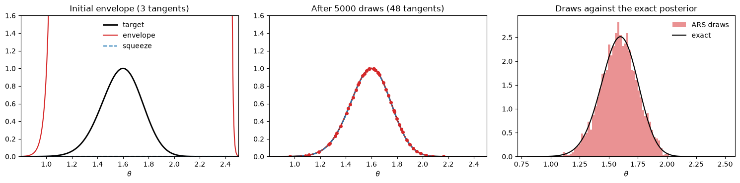
The envelope starts loose, so early draws are often rejected and each rejection teaches it a tangent. After a few dozen evaluations it hugs the target, the squeeze accepts almost every draw without touching the target, and the remaining thousands of draws cost essentially nothing. Refining the envelope never affects exactness: every accepted draw is exact whatever the envelope looks like at the time.

2. Rejection sampling with a learned bound¶

For a multivariate target, rejection takes any proposal with heavier tails. The target here is a banana, \(x_1 \sim \mathcal N(0, 2^2)\), \(x_2 \mid x_1 \sim \mathcal N(x_1^2/2 - 2, 0.5^2)\), and the proposal a broad Gaussian. \(\log M\) is unknown, so the kernel starts with \(\log M = -\infty\) and its default adaptation, bound_adaptor, raises it to the largest \(\log p - \log q\) seen during warmup. Each step's info reports the largest ratio among its proposals, so a bound that is still too low shows up as max_log_ratio > log_bound.

def banana(x):
    return -0.5 * (x[0] ** 2 / 4 + (x[1] - 0.5 * x[0] ** 2 + 2) ** 2 / 0.25)


broad = Density(
    sample=lambda key, scale: scale * jax.random.normal(key, (2,)),
    logpdf=lambda x, scale: jax.scipy.stats.norm.logpdf(x, 0.0, scale).sum(),
)
kernel = rejection(banana, proposal=broad)
state = kernel.init(jax.random.key(0), jnp.zeros(2))
params = kernel.init_params(state, 4.0)

tuned = warmup(jax.random.key(1), kernel, state, params, 2000)
gaussian_draws = run(jax.random.key(2), kernel, tuned.state, tuned.params, 5000,
                     collect=("position", "num_proposals", "max_log_ratio")).trace


def report(name, trace, log_bound):
    violations = int((trace["max_log_ratio"] > log_bound).sum())
    lag_one = jnp.corrcoef(trace["position"][:-1, 0], trace["position"][1:, 0])[0, 1]
    print(f"{name:>16}: log M = {float(log_bound):5.2f}, proposals per draw = "
          f"{trace['num_proposals'].mean():5.1f}, steps exceeding the bound = {violations}, "
          f"lag-1 autocorrelation = {lag_one:+.3f}")


gaussian_bound = tuned.params.log_bound
report("Gaussian q", gaussian_draws, gaussian_bound)

      Gaussian q: log M =  7.11, proposals per draw = 197.3, steps exceeding the bound = 2, lag-1 autocorrelation = +0.021

The draws are independent: the lag-1 autocorrelation is zero up to noise, where an MCMC chain would show strong correlation. The cost moves into the number of proposals per draw, which is \(M\) times the ratio of normalising constants: a broad Gaussian wastes most proposals in the empty space around the banana. A small number of steps exceeding the bound means warmup saw nearly, but not exactly, the largest ratio. Those draws are slightly over-represented, so warm up longer or pass bound_adaptor(margin=...) when that matters.

3. A learned flow proposal¶

A proposal that matches the target needs far fewer proposals per draw. The accepted draws are exact target samples, so they are exactly the right data for training a flow by maximum likelihood. fit_adaptor(field="proposal") does that inside the scan, composed with bound_adaptor so the bound keeps up. The flow starts broad (standardization scale 4).

flow = maf(2, 3, rngs=nnx.Rngs(0))
flow.set_standardization(jnp.zeros(2), 4.0 * jnp.ones(2))
proposal, proposal_params = density(flow)

kernel = rejection(banana, proposal=proposal)
state = kernel.init(jax.random.key(0), jnp.zeros(2))
policy = compose_adaptors(
    proposal=fit_adaptor(maximum_likelihood(proposal), optax.adam(3e-3), field="proposal"),
    bound=bound_adaptor(),
)

start = time.perf_counter()
trained = run(jax.random.key(1), kernel, state, kernel.init_params(state, proposal_params), 3000,
              adaptor=policy, collect=("num_proposals",))
print(f"training: {time.perf_counter() - start:.1f}s, log M after training = {float(trained.params.log_bound):.2f}")

training: 0.5s, log M after training = 6.13

The bound only ever grows, so after training it still reflects the poor early proposals and is far too loose for the trained flow: the number of proposals per draw stays high (left panel below). The remedy is a second, short phase: keep the trained flow fixed and learn the bound afresh.

fresh = trained.params._replace(log_bound=jnp.asarray(-jnp.inf))
tuned = warmup(jax.random.key(2), kernel, trained.state, fresh, 2000)
flow_draws = run(jax.random.key(3), kernel, tuned.state, tuned.params, 5000,
                 collect=("position", "num_proposals", "max_log_ratio")).trace

report("Gaussian q", gaussian_draws, gaussian_bound)
report("trained flow q", flow_draws, tuned.params.log_bound)

      Gaussian q: log M =  7.11, proposals per draw = 197.3, steps exceeding the bound = 2, lag-1 autocorrelation = +0.021
  trained flow q: log M =  3.30, proposals per draw =   4.4, steps exceeding the bound = 8, lag-1 autocorrelation = -0.026

xs, ys = jnp.meshgrid(jnp.linspace(-7, 7, 200), jnp.linspace(-4, 12, 200))
log_banana = jax.vmap(jax.vmap(lambda a, b: banana(jnp.array([a, b]))))(xs, ys)

fig, axes = plt.subplots(1, 3, figsize=(15, 3.8))
window = 100
axes[0].plot(jnp.convolve(trained.trace["num_proposals"], jnp.ones(window) / window, mode="valid"),
             color="tab:green")
axes[0].axhline(flow_draws["num_proposals"].mean(), color="tab:green", ls="--", label="after re-learning the bound")
axes[0].axhline(gaussian_draws["num_proposals"].mean(), color="tab:orange", ls="--", label="Gaussian q")
axes[0].set(xlabel="training step", ylabel="proposals per draw (running mean)", yscale="log",
            title="Training with a growing bound")
axes[0].legend(frameon=False, fontsize=8)

flow_samples = jax.vmap(proposal.sample, (0, None))(jax.random.split(jax.random.key(4), 3000), tuned.params.proposal)
for ax, points, color, title in [
    (axes[1], flow_samples, "tab:green", "Trained flow $q$ (approximate)"),
    (axes[2], flow_draws["position"][:3000], "tab:red", "Rejection draws (exact, iid)"),
]:
    ax.contour(xs, ys, log_banana, levels=[-8, -4.5, -2, -0.5], colors="0.6", linewidths=0.8)
    ax.scatter(*points.T, s=1, alpha=0.4, color=color, rasterized=True)
    ax.set(xlim=(-7, 7), ylim=(-4, 12), title=title)
plt.tight_layout()
plt.show()

png

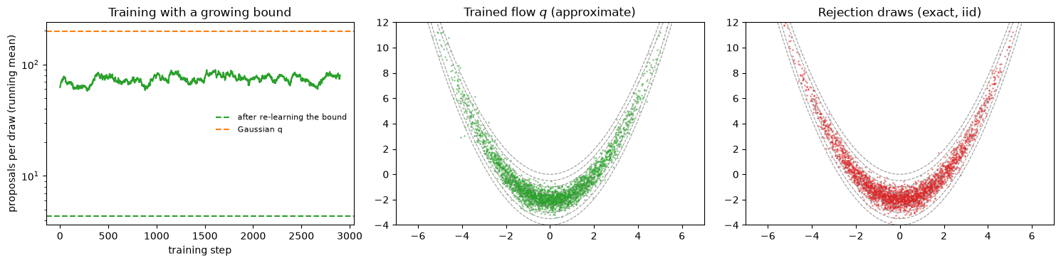
With the bound re-learned, the trained flow needs a fraction of the proposals the broad Gaussian needs, and every accepted draw is still exact: the flow's own mistakes (its samples are visibly off in the tips of the banana) are corrected by the accept step, not inherited.

When to use what¶

Situation	Use
Univariate, log-concave (conditionals in a Gibbs sampler, GLM posteriors per coordinate)	`ars`: exact, and nearly free once the envelope is tight
Univariate, not log-concave	`arms` (an MCMC kernel on the same envelope)
Low dimension, a proposal with heavier tails is available	`rejection` with `bound_adaptor` warmup
The proposal is poor	Train a flow with `fit_adaptor(field="proposal")`, then re-learn the bound with the flow fixed
High dimension	MCMC: the proposals needed per draw grow exponentially with dimension

Caveats:

The bound has to be a bound. Draws are exact only where \(\log p - \log q \le \log M\). bound_adaptor learns \(\log M\) from what it sees, so check max_log_ratio against log_bound on the draws you keep, and give the proposal heavier tails than the target, or no finite bound exists at all.
Freeze adaptation for the draws you report, as with MCMC: a bound that is still growing over-represents the regions where it was too low.